Difference between Algorithm Paradigms

Written by:

Fagun Shadi D-53

Tejas Shantaram D-71

Shruti Vasave D-76

Vidhi Raghvani D-77

Greedy Algorithmic Paradigm:

Greedy is an algorithmic paradigm that creates up an answer part by part, always choosing a subsequent part that gives the foremost obvious and immediate benefit. So, the issues where choosing locally optimal also results in global solution are best fit Greedy. A number of steps form the solution. At every step the best possible step, or solution, was selected. This process was repeated at every step till the solution was found. This is not the most optimal solution, but instead finds the best solution at every step, like a local minima. Greedy breaks the problem into sub-problems. And each sub problem is solved to the best possible way using Greedy paradigm. All sub problems are solved from the top down. The Problems are reduced step by step, and the solution is obtained when the whole problem goes away.

Dynamic Programming:

Dyanamic Programming is an optimisation on recursion algorithm. Recursive solutions have repeated calls for same inputs. This can easily be optimised by Dynamic Programming. As with every other algorithmic paradigm, every problem is broken into sub-problems. In each sub-problem, the results are stored, to reduce the number of re-computations required at each step. These Optimizations at each level, help us to save trips back to get results, and thus reduce the time complexities from exponential to polynomial. If we take the example of Fibonacci numbers, the simple recursive solution is exponential time complexity. However, we can optimise the problem by storing the solutions at each level, and thus reduce the time complexity to linear.

Divide and Conquer:

In Divide and conquer, we split the big problem into smaller sub-problems, which are identical to the big problem. That is, they are small versions of the same problem. We then find the solution for the sub-problems and then combine all the solutions to solve the bigger problem! A classic example of divide and conquer is eating a big chocolate bar. We can split the chocolate bar into smaller piece, enjoy each piece and thus eat the whole chocolate bar step by step.

Difference between the three:

Dynamic Programming solves the sub-problems bottom up. The problem can’t be solved until we find all solutions of sub-problems. The solution comes up when the whole problem appears. Greedy solves the sub-problems from top down. We first need to find the greedy choice for a problem, then reduce the problem to a smaller one. The solution is obtained when the whole problem disappears.

 Dynamic Programming has to try every possibility before solving the problem. Itis much more expensive than greedy. However, there are some problems that greedy cannot solve while dynamic programming can. Therefore, we first try greedy algorithm. If it fails, then try dynamic programming

Divide-&-conquer works best when all sub-problems are independent. So, pick partition that makes algorithm most efficient & simply combine solutions to solve entire problem.

Dynamic programming is needed when subproblems are dependent; we don’t know where to partition the problem.

Divide-&-conquer is best suited for the case when no “overlapping sub-problems” are encountered. In dynamic programming algorithms, we typically solve each subproblem only once and store their solutions. But this is at the cost of space.

GREEDY ALGORITHM AND ITS APPLICATIONS

Written by:

Fagun Shadi D-53

Tejas Shantaram D-71

Shruti Vasave D-76

Vidhi Raghvani D-77

 The Greedy Property:
                    "make a choice that seems best at the moment then solve sub problems that arise later".

The greedy algorithms are based on this certain property. Greedy algorithms are in fact greedy. 

They're concerned with what the global optimal solution is therein very moment instead of looking into the longer term . This suggests that the general optimal solution could be different from the answer that the algorithm chooses at the start .

This is actually the main difference between greedy strategy and dynamic programming - in dynamic programming, all sub problems are solved, then one among them is chosen to find the optimal solution. Whereas greedy algorithms never optimize globally.

Greedy algorithms can’t always guarantee solutions, but they're very time efficient. We’ll also see later how sometimes greedy strategy solutions do give optimal solutions.

What are greedy algorithms used for ?

As we talked about earlier, greedy algorithms are very time efficient; in order that they are pretty fast in comparison to the opposite alternatives - Divide and conquer or dynamic programming .

Not all, but there are a couple of algorithms that are known to offer globally optimal solutions every time. Let’s have a glance at what these algorithms are.

• Dijkstra’s algorithm
• Kruskal’s algorithm
•  Prim’s algorithm
•  Huffman trees

Let’s explore these greedy algorithms. 

Dijkstra’s algorithm  

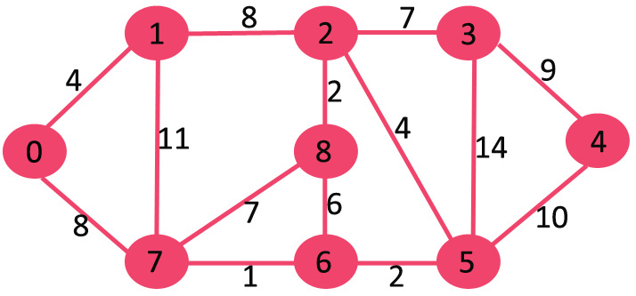
This algorithm is especially used to solve any shortest distance problem. For instance, the shortest distance between two points on a graph or shortest routes.

Dijkstra’s algorithm has a lot of uses. They are often very useful within road networks where you would like to seek out the fastest and shortest route to an area .

Other places where this algorithm is used include IP Routing, A*Algorithm, Telephone networks, etc.

Dijkstra's Algorithm

Kruskal’s Algorithm

This algorithm solves the problem of finding a Minimum Spanning Tree (MST) of any connected and undirected graph.

Kruskal’s is a greedy approach that mainly emphasizes on the very fact that we must include only those edges in our MST that have minimum weight among all of them, ensuring that we don't include those edges that make a cycle in MST being constructed.

Kruskal's Algorithm

Prim’s Algorithm

Prim’s algorithm is a slightly different approach than Kruskal’s. It's another greedy algorithm that finds a minimal spanning tree in a connected, weighted graph.

As we see in Kruskal’s, the partial solutions aren't connected usually, but in Prim’s the partial solution is a tree.

The greedy rule applied in Prims algorithm “Add an edge of minimum weight that has one vertex within the current tree and therefore the other not within the current tree.

Prim's Algorithm

Huffman Trees

Huffman Tree is full binary tree in which each leaf of the tree corresponds to a letter within the given alphabet. It's a data compression algorithm which uses the greedy strategy.

The greedy rule applied here is: "at each iteration, the algorithm makes a “greedy” decision to merge the 2 subtrees with least weight."

Huffman Trees

A few Algorithmic Paradigms

Written by:

Fagun Shadi D-53

Tejas Shantaram D-71

Shruti Vasave D-76

Vidhi Raghvani D-77 

Greedy Algorithmic Paradigm

The greedy algorithm first appeared in the combinatorial optimization literature in a 1971 article by Edmonds but the foundation of this algorithm was laid in 1935 in Whitney’s dissertation on the Theory of Matroids. Greedy Algorithm is essentially a simple and intuitive algorithm to solve optimization problems. Generally, an optimization problem follows certain steps with some choices at each step. A greedy algorithm chooses the step that gives the most locally optimal choice. It is important to note that it is possible that the Greedy algorithm may not fulfil the intent of finding a global optimal solution. Despite this, greedy method provides to be quite powerful and works for a large range of problems which this blog will subsequently cover.

In any optimization problem, time complexity plays an important role in determining the efficiency of the algorithm. Greedy algorithms are generally faster as they provide local optimal solutions. Another important factor to determine efficiency is memory requirement. Greedy algorithms have less memory requirement as they don’t revise or go back to the choices they made earlier. While in case of dynamic programming, it needs a dp table to store the choices and make changes if needed. Thus, Greedy algorithms are more efficient than Dynamic Programming.

A greedy algorithm, always makes the selection that seems to be the simplest at that moment. This means that it makes a choice that is optimal in that local sense with the hope that this choice will cause a globally-optimal solution.

How do you decide which choice is optimal?

Assume that you simply have an objective function that must be optimized (either maximized or minimized) at a given point. A Greedy algorithm makes greedy choices at each step to make sure that the target function is optimized. The Greedy algorithm has just one shot to compute the optimal solution in order that it never goes back and reverses the choice.

There will be certain times when we have to make a decision which affects the state of the system, which may or may not be known to us in advance. These decisions or changes are like transformations of state variables. The results of the previous decisions help us in choosing the long term ones.

What do we conclude from this? We need to cut up a main problem into a series of overlapping sub-problems, and build up solutions to larger and bigger sub-problems. If you're given a prob statement which may be weakened into smaller sub-problems, and these smaller sub-problems can still be broken into smaller ones - and if you manage to discover some over-lapping sub-problems, then you’ve encountered a DP problem.

Dynamic Programming 

The core idea of Dynamic Programming is to avoid repeated work by remembering partial results and this idea finds it application during a lot of real-life situations.

1. Frame the optimization problem such that after a local optimum solution is selected only one sub problem remains

2. Show that there is always some solution that is optimal to the original problem that makes the greedy choice, so that the greedy choice is always safe.

3. Show that once a choice is made according to the greedy method, the sub problem that remains is such that if we combine an optimal solution to the sub problem, we will get an optimal solution to the original problem